44 excel data labels scatter plot
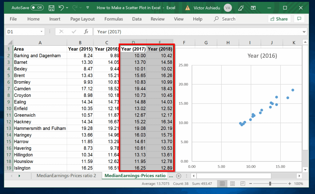
Macro to add data labels to scatter plot - MrExcel Message Board It's an Excel macro, not something that requires installing. Downloading, yes, but you can put the macro anywhere. In any case, here's the code: Sub AddXYLabels () If Left (TypeName (Selection), 5) <> "Chart" Then MsgBox "Please select the chart first." Exit Sub End If Set StartLabel = _ how to make a scatter plot in Excel — storytelling with data Select "Scatter" from the options in the "Recommended Charts" section of your ribbon. Excel will automatically create a scatter plot for you in the same sheet as your data, using the first column of your dataset as the horizontal (X) axis, and the second column as your vertical (Y) axis.
How to add data labels from different column in an Excel chart? This method will guide you to manually add a data label from a cell of different column at a time in an Excel chart. 1. Right click the data series in the chart, and select Add Data Labels > Add Data Labels from the context menu to add data labels. 2.
Excel data labels scatter plot
How to use a macro to add labels to data points in an xy scatter chart ... In Microsoft Office Excel 2007, follow these steps: Click the Insert tab, click Scatter in the Charts group, and then select a type. On the Design tab, click Move Chart in the Location group, click New sheet , and then click OK. Press ALT+F11 to start the Visual Basic Editor. On the Insert menu, click Module. › examples › data-seriesChart's Data Series in Excel - Easy Tutorial Select Data Source. To launch the Select Data Source dialog box, execute the following steps. 1. Select the chart. Right click, and then click Select Data. The Select Data Source dialog box appears. 2. You can find the three data series (Bears, Dolphins and Whales) on the left and the horizontal axis labels (Jan, Feb, Mar, Apr, May and Jun) on ... How to Make a Scatter Plot in Excel? 4 Easy Steps - Simon Sez IT Option 1: Plot both variables in X vs Y scatter plot style. Use this option to check for linear relationships between variables. To implement this, just select the range of the two variables. Option 1: Select the two continuous variables. Option 2 involves plotting the variables separately in two different series.
Excel data labels scatter plot. Labels for data points in scatter plot in Excel - Microsoft Community The points have been created on my scatter plot and I would like to label the points with the events listed in a column in my table. I see in Label Options where I can have the label contain the X value and/or Y value, but not anything else (except Series Name). Prevent Overlapping Data Labels in Excel Charts - Peltier Tech Apply Data Labels to Charts on Active Sheet, and Correct Overlaps Can be called using Alt+F8 ApplySlopeChartDataLabelsToChart (cht As Chart) Apply Data Labels to Chart cht Called by other code, e.g., ApplySlopeChartDataLabelsToActiveChart FixTheseLabels (cht As Chart, iPoint As Long, LabelPosition As XlDataLabelPosition) How to create a scatter plot and customize data labels in Excel During Consulting Projects you will want to use a scatter plot to show potential options. Customizing data labels is not easy so today I will show you how th... Add or remove data labels in a chart - support.microsoft.com Add data labels to a chart Click the data series or chart. To label one data point, after clicking the series, click that data point. In the upper right corner, next to the chart, click Add Chart Element > Data Labels. To change the location, click the arrow, and choose an option.
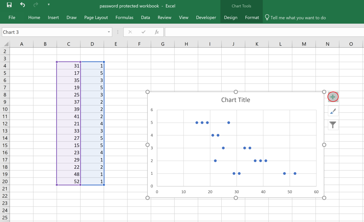
How to Create Scatter Plots in Excel (In Easy Steps) To create a scatter plot with straight lines, execute the following steps. 1. Select the range A1:D22. 2. On the Insert tab, in the Charts group, click the Scatter symbol. 3. Click Scatter with Straight Lines. Note: also see the subtype Scatter with Smooth Lines. Note: we added a horizontal and vertical axis title. How to find, highlight and label a data point in Excel scatter plot Add the data point label To let your users know which exactly data point is highlighted in your scatter chart, you can add a label to it. Here's how: Click on the highlighted data point to select it. Click the Chart Elements button. Select the Data Labels box and choose where to position the label. How to Add Labels to Scatterplot Points in Excel - Statology Step 3: Add Labels to Points. Next, click anywhere on the chart until a green plus (+) sign appears in the top right corner. Then click Data Labels, then click More Options…. In the Format Data Labels window that appears on the right of the screen, uncheck the box next to Y Value and check the box next to Value From Cells. How to label scatterplot points by name? - Stack Overflow 13 Apr 2016 — right click on your data point · select "Format Data Labels" (note you may have to add data labels first) · put a check mark in "Values from Cells ...5 answers · Top answer: Well I did not think this was possible until I went and checked. In some previous version of ...How to label scatter point plots from data column in excel23 Jul 2017Use text as horizontal labels in Excel scatter plot - Stack ...11 Jun 2017Excel: labels on a scatter chart, read from array - Stack Overflow29 Jan 2015Excel data representation, Axis labelling non-numeric - Stack ...6 Oct 2020More results from stackoverflow.com
Scatter Plot not showing all data points - Excel Help Forum I created a scatter plot based on a table with 25 data coordinates but (1) only 16 coordinates are showing in the scatter plot and (2) some of the labels on the scatter plot aren't showing. Does anyone know how I can fix this? Images are below. Here's some other information that might be useful: - I'm using Excel for Mac 2019 (standalone version). How to add conditional colouring to Scatterplots in Excel Step 3: Edit the colours. To edit the colours, select the chart -> Format -> Select Series A from the drop down on top left. In the format pane, select the fill and border colours for the marker. Repeat these steps for Series B and Series C. Here is our final scatterplot. How to Quickly Add Data to an Excel Scatter Chart Right-click the chart and choose Select Data. Click Add above the bottom-left window to add a new series. In the Edit Series window, click in the first box, then click the header for column D. This time, Excel won't know the X values automatically. Click inside the box below Series X values, then select the X data (either click and drag or ... Add Custom Labels to x-y Scatter plot in Excel Step 1: Select the Data, INSERT -> Recommended Charts -> Scatter chart (3 rd chart will be scatter chart) Let the plotted scatter chart be. Step 2: Click the + symbol and add data labels by clicking it as shown below. Step 3: Now we need to add the flavor names to the label. Now right click on the label and click format data labels.
Scatter Plot Template in Excel | Scatter Plot Worksheet
Scatter Graph - Overlapping Data Labels - Excel Help Forum We are not able to work with or manipulate a picture of one and nobody wants to have to recreate your data from scratch. 1. Make sure that your sample data are REPRESENTATIVE of your real data. The use of unrepresentative data is very frustrating and can lead to long delays in reaching a solution. 2.
How to Create a Scatter Plot in Excel - TurboFuture - Technology
How to Find, Highlight, and Label a Data Point in Excel Scatter Plot? By default, the data labels are the y-coordinates. Step 3: Right-click on any of the data labels. A drop-down appears. Click on the Format Data Labels… option. Step 4: Format Data Labels dialogue box appears. Under the Label Options, check the box Value from Cells . Step 5: Data Label Range dialogue-box appears.

How to join the points on a scatter plot in Excel - YouTube
Improve your X Y Scatter Chart with custom data labels Select the x y scatter chart. Press Alt+F8 to view a list of macros available. Select "AddDataLabels". Press with left mouse button on "Run" button. Select the custom data labels you want to assign to your chart. Make sure you select as many cells as there are data points in your chart. Press with left mouse button on OK button. Back to top
How to Make a Scatter Plot in Excel | Itechguides.com
Use text as horizontal labels in Excel scatter plot Edit each data label individually, type a = character and click the cell that has the corresponding text. This process can be automated with the free XY Chart Labeler add-in. Excel 2013 and newer has the option to include "Value from cells" in the data label dialog. Format the data labels to your preferences and hide the original x axis labels.
How to separate overlapping data points in Excel - YouTube
How to Create a Scatterplot with Multiple Series in Excel Step 3: Create the Scatterplot. Next, highlight every value in column B. Then, hold Ctrl and highlight every cell in the range E1:H17. Along the top ribbon, click the Insert tab and then click Insert Scatter (X, Y) within the Charts group to produce the following scatterplot: The (X, Y) coordinates for each group are shown, with each group ...

Fors: Adding labels to Excel scatter charts
Custom Data Labels for Scatter Plot | MrExcel Message Board sub formatlabels () dim s as series, y, dl as datalabel, i%, r as range set r = [j5] set s = activechart.seriescollection (1) y = s.values for i = lbound (y) to ubound (y) set dl = s.points (i).datalabel select case r case is = "won" dl.format.textframe2.textrange.font.fill.forecolor.rgb = rgb (250, 250, 5) dl.format.fill.forecolor.rgb = rgb …
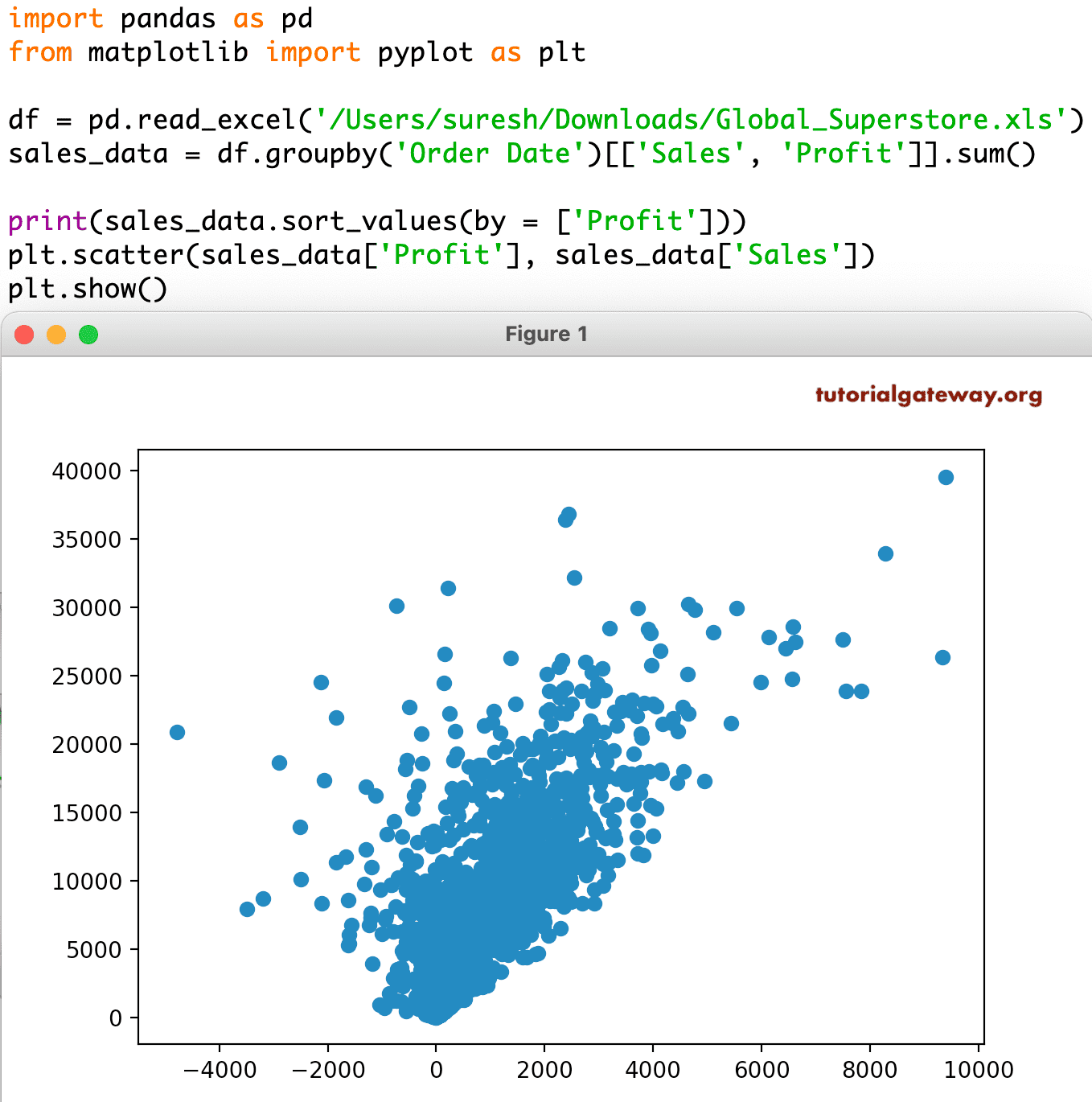
Python matplotlib Scatter Plot
How to Make a Scatter Plot in Excel | GoSkills Create a scatter plot from the first data set by highlighting the data and using the Insert > Chart > Scatter sequence. In the above image, the Scatter with straight lines and markers was selected, but of course, any one will do. The scatter plot for your first series will be placed on the worksheet. Select the chart.
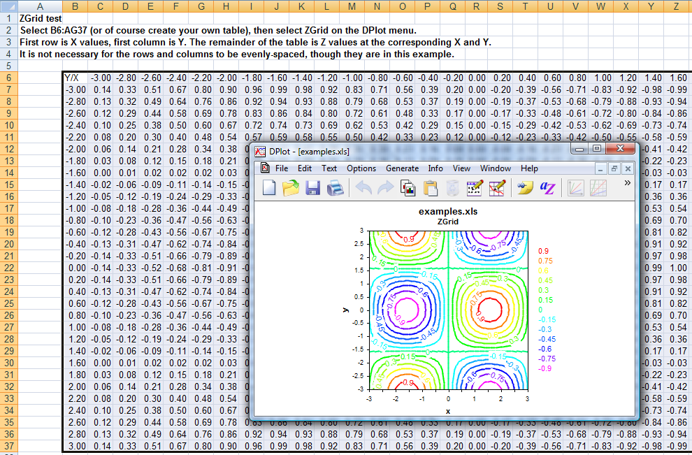
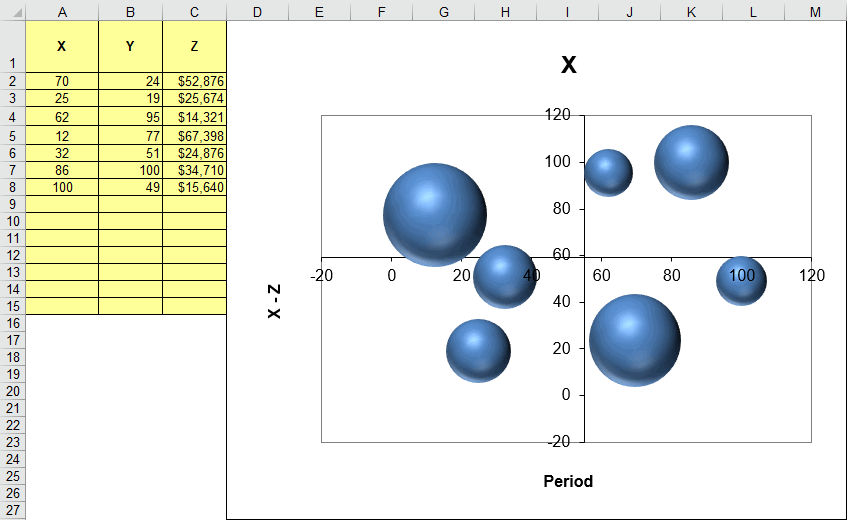
Getting Started > Getting Started with XYZ Surface Plots > Getting Started with XYZ Surface ...
How to display text labels in the X-axis of scatter chart in Excel? Display text labels in X-axis of scatter chart Actually, there is no way that can display text labels in the X-axis of scatter chart in Excel, but we can create a line chart and make it look like a scatter chart. 1. Select the data you use, and click Insert > Insert Line & Area Chart > Line with Markers to select a line chart. See screenshot: 2.
Post a Comment for "44 excel data labels scatter plot"